斯坦福ML课程——python转写(Week3—课程作业ex2_1)

利用python完成课程作业ex2的第一部分，第一部分的要求如下（具体要求：https://www.coursera.org/learn/machine-learning/home/week/3）：

In this part of the exercise, you will build a logistic regression model to predict whether a student gets admitted into a university. Suppose that you are the administrator of a university department and you want to determine each applicant's chance of admission based on their results on two exams. You have historical data from previous applicants that you can use as a training set for logistic regression. For each training example, you have the applicant's scores on two exams and the admissions
decision. Your task is to build a classication model that estimates an applicant's probability of admission based the scores from those two exams. This outline and the framework code in ex2.m will guide you through the exercise.

在ex2.m的代码中，分为四个部分，每个部分分别如下：

1. Part 1: Plotting #显示课程给出的数据
2. Part 2: Compute Cost and Gradient #计算cost以及gradient
3. Part 3: Optimizing using minimize #进行优化，课程中给出的是利用fminunc，python中我用的是minimize
4. Part 4: Predict and Accuracies #预测和准确度

由于我现在是只想单纯地去实现这个练习，所以没有考虑算法的整体结构，实用性和可读性，即部分是没有定义函数的，输出的时候也没有明确的指示，在完成整个作业之后会重新对算法进行进一步的修改。以下是我的代码：

"""
Created on Mon Nov 11 07:50:44 2019

@author: Lonely_hanhan
"""

import numpy as np
import matplotlib.pyplot as plt
import scipy.optimize as op
from mpl_toolkits.mplot3d import Axes3D

"""
加载数据&显示数据
"""
Data = np.loadtxt('D:\exercise\machine-learning-ex2\ex2\ex2data1.txt', delimiter=',')
X = Data[:,0:2]
[m,n] = X.shape
Y = Data[:,2] #此处读取的时一维数组，需转化为m维数组
Y = Y.reshape((m,1))

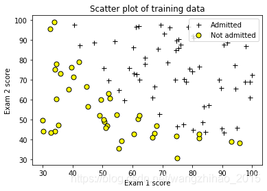
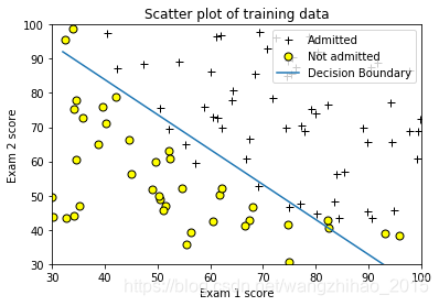
''' ==================== Part 1: Plotting ==================== '''

pos = np.where(Y == 1)
neg = np.where(Y == 0)

#由于Y为二维数组，所以where得到的值都为tuple类型，需提取行坐标

p = pos[0].shape[0]
pos = pos[0].reshape(p, 1) #Y值为1的下标位置
ne = neg[0].shape[0]
neg = neg[0].reshape(ne, 1) #Y值为0的下标位置

plt.plot(X[pos, 0], X[pos, 1], color='black', linewidth='2', marker='+', markersize='7', markerfacecolor = 'black', linestyle='None')
plt.plot(X[neg, 0], X[neg, 1], color='black', marker='o', markersize='7',markerfacecolor = 'yellow', linestyle='None')

#设置标题，横纵坐标 图例

plt.title('Scatter plot of training data')
plt.xlabel('Exam 1 score')
plt.ylabel('Exam 2 score')
plt.legend(('Admitted', 'Not admitted'), loc='upper right')
plt.show()
"""
需要在X中加入x0，即列向量加上数值为1的m维向量，即n+1
"""
x_0 = np.ones((m,1))
X = np.hstack((x_0, X))
initial_theta = np.zeros((1, n + 1))

''' ==================== Part 2: Compute Cost and Gradient ==================== '''
#创建h(x)函数
def h_func(z):
    return 1/(1+np.exp(-z))
#创建损失函数
def costFunction(theta, X, Y):
    jVal = (-np.dot(np.log(h_func(np.dot(theta, X.T))), Y) - np.dot(np.log(1 - h_func(np.dot(theta, X.T))), (1-Y))) / m
    return jVal
#创建梯度函数
def gradient(theta, X, Y):
    grad = np.dot((h_func(np.dot(theta, X.T))-Y.T), X) / m
    return grad

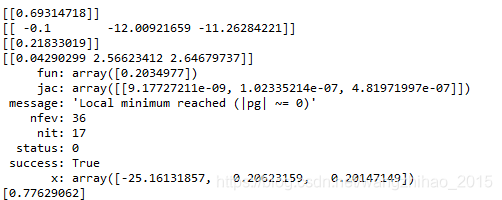
cost1 = costFunction(initial_theta, X, Y)
print(cost1)
grad1 = gradient(initial_theta, X, Y)
print(grad1)

test_theta =np.array([[-24, 0.2, 0.2]])
cost2 = costFunction(test_theta, X, Y)
print(cost2)
grad2 = gradient(test_theta, X, Y)
print(grad2)

''' ==================== Part 3: Optimizing using minimize ==================== '''

result = op.minimize(fun=costFunction, x0=initial_theta, args=(X, Y), method='TNC', jac=gradient, options= {'maxiter': 400})
print(result)

# plot boundary
# 映射为多项式 ,该函数需结合matlab中help mapFeature进行看，引用了https://github.com/hujinsen/python-machine-learning
# 中5.映射为多项式
def mapFeature(X1,X2):
    degree = 3;                     # 映射的最高次方
    out = np.ones((X1.shape[0],1))  # 映射后的结果数组（取代X）
    '''
    这里以degree=2为例，映射为1,x1,x2,x1^2,x1,x2,x2^2
    '''
    for i in np.arange(1,degree+1): 
        for j in range(i+1):
            temp = X1**(i-j)*(X2**j)    #矩阵直接乘相当于matlab中的点乘.*
            out = np.hstack((out, temp.reshape(-1,1)))
    return out

#plot data
    
plt.plot(X[pos, 1], X[pos, 2], color='black', linewidth='2', marker='+', markersize='7', markerfacecolor = 'black', linestyle='None')
plt.plot(X[neg, 1], X[neg, 2], color='black', marker='o', markersize='7',markerfacecolor = 'yellow', linestyle='None') 

if X.shape[1] <= 3:
    plot_x = np.array([np.max(X[:,1])-2, np.min(X[:,1])+2]) #Only need 2 points to define a line, so choose two endpoint
    plot_y = (-1/result.x[2])*(result.x[1]*plot_x + result.x[0])# Calculate the decision boundary line，即计算exam2的值
    plt.plot(plot_x, plot_y)
    plt.legend(('Admitted', 'Not admitted', 'Decision Boundary'), loc='upper right')
    plt.axis([30, 100, 30, 100])
else:
    '''
    这一部分需要进一步研究
    '''    
    # Here is the grid range
    u = np.linspace(-1, 1.5, 50)
    v = np.linspace(-1, 1.5, 50)
    z = np.zeros([len(u), len(u)])
    for i in range(1,len(u)):
        for j in range(1,len(v)):
            z[i,j] = mapFeature(u(i), v(j))*result.x;
    z = z.T; # important to transpose z before calling contour
    fig = plt.figure()
    ax = Axes3D(fig)
    ax.plot_surface(u, v, z, rstride=1, cstride=1, cmap='rainbow')

plt.title('Scatter plot of training data')
plt.xlabel('Exam 1 score')
plt.ylabel('Exam 2 score')    


''' ==================== Part 4: Predict and Accuracie==================== '''
#  After learning the parameters, you'll like to use it to predict the outcomes
#  on unseen data. In this part, you will use the logistic regression model
#  to predict the probability that a student with score 45 on exam 1 and 
#  score 85 on exam 2 will be admitted.
#
#  Furthermore, you will compute the training and test set accuracies of 
#  our model.
# Predict probability for a student with score 45 on exam 1  and score 85 on exam 2 
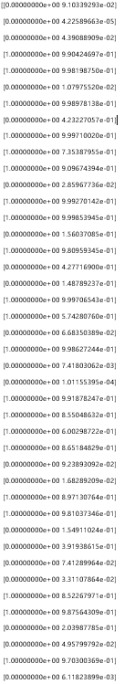
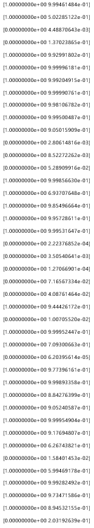
S = np.array([[1, 45, 85]])
p = h_func(np.dot(result.x, S.T))#y为1的概率值
print(p)

y_p = np.zeros(shape=(m,2))

for i in range(0, m):
    XT = X[i,:].reshape((-1,1))
    y_p[i,1] = h_func(np.dot(result.x, XT))
    if h_func(np.dot(result.x, XT)) > 0.5:
        y_p[i,0] = 1
    else:
        y_p[i,0] = 0
print(y_p)
            

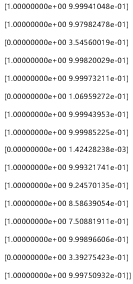
运行结果如下：

在书写代码的过程中，本文借鉴了以下几位大佬：

对于minimize函数，     作者：csdn_inside 链接：https://www.twblogs.net/a/5bf35646bd9eee37a142e45a/zh-cn

对于mapFeature函数，作者：JSen            链接：https://github.com/hujinsen/python-machine-learning

为了记录自己的学习进度同时也加深自己对知识的认知，刚刚开始写博客，如有错误或者不妥之处，请大家给予指正。